Building designers are increasingly being asked to assess how their buildings will perform in future climate conditions. To help with future building performance assessments, organisations such as CIBSE and CSIRO have issued sets of ‘future weather years’ for building simulation that take into account the impact of various projected climate change scenarios. These are based on a series of standard assumptions related to human economic and population growth and the effectiveness of the political and technical solutions applied. Future weather files can be used instead of the usual historical weather data in building models to assess future building performance.
Because future weather files are provided for a range of scenarios and future periods, it makes sense to run simulations for the range of scenarios all in one go and to display results for all files on a single page. DesignBuilder's parametric analysis tools are ideal for this. This tutorial explains all of the steps involved in generating parametric outputs for future weather files.
Tip: A similar approach can be taken for running batch simulations for any controlled set of variations in weather files, such as for a range of actual weather years to ensure that all historic weather conditions are covered (rather than using 1 "typical" weather year).
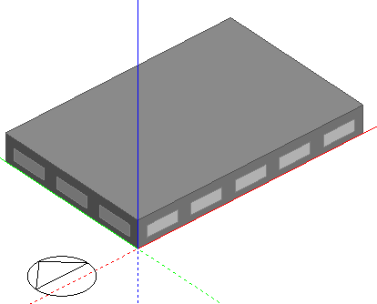
Create a new file located in London Gatwick and add a building to the site with a simple rectangular block having dimensions 30m x 20m as shown below.
Navigate to building level and make the following changes to the base model to use a simple heating system with natural ventilation and to minimise internal and solar gains to levels that are perhaps more realistic in future buildings:
On the HVAC tab select the Radiator heating, Boiler HW, Mech vent Supply + Extract template.
Still on the HVAC tab set the Natural Ventilation, Outside air flow rate to 10 ac/h.
On the Opening tab switch on Local shading and select 1m overhangs.
On the Lighting tab select the LED with linear control Lighting template.
On the Activity tab set the power density for Office equipment to be 8 W/m2.
On the Constructions tab select the Best practice heavyweight template.
Click on the Simulation tab and run a base annual simulation.
On the calculation options dialog, first select the 2-Operative temperature control method to help the comfort assessment methods avoid reporting underheating in winter.
Because it is a simple model you can select hourly results. Make sure to also choose Monthly results which are required by the Optimisation.
Then run the simulation.
Check the hourly results for the simulation period and make sure that the model is behaving as expected, including temperatures within the building, comfort levels, operations periods etc. If necessary fix the model and repeat this step until you are happy with the base model hourly results.
Now run a final simulation without hourly and daily results but with Monthly and Run period results to prepare the model for the parametric analysis.
To follow the exact steps in this example you will need access to the CIBSE weather files for London. However you can use any future files suitable for your location, but do make sure that the weather files are for more or less the same location as the rest of the location data set at site level.
You can obtain the CIBSE weather files from the DesignBuilder website.
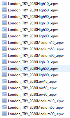
Once you have downloaded the weather files, you must extract the data from the zip file and copy all of the required epw files to the DesignBuilder Weather folder. You can open Windows Explorer at this location through the File > Folders > Weather Data menu command. You should end up with these files in the Weather Data folder.
The next step is to create a new Hourly weather data component for each of the 18 weather files to be analysed. This can be done by following the steps explained in Add New hourly weather data. To summarise:
Open the Select Hourly weather data browse dialog.
Take a copy of the Default London Hourly weather data component by selecting it and pressing the Create copy of highlighted item button.
Edit the copy by selecting it and pressing the Edit selected data icon.
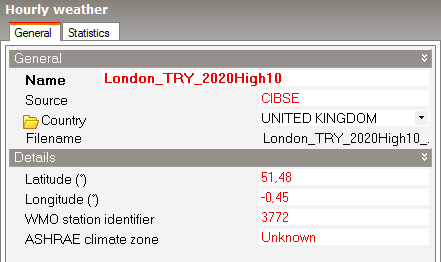
On the Edit hourly weather dialog start by selecting the first file in the list, London_TRY_2020High10_.epw. Copy the file name minus the .epw extension and use the text as the name of the Hourly weather component by pasting the copied text into the Name field. You might also like to enter the Source as "CIBSE" but that is optional The dialog should now look something like this:
Now repeat the process for the remaining 17 weather files. Be sure to follow the process carefully in a systematic way to avoid errors.
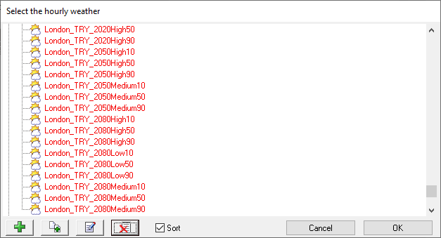
When you've finished the list of Hourly weather data should look like this:
Once you have a good understanding of how the base model operates, especially during warm summer periods, you are ready to start the parametric analysis stage.
For this simple example we will investigate the effect of changing the hourly weather file on building discomfort.
To do that follow these steps.
Step 5.a - Open the Parametric, Optimisation and UA/SA Analysis Settings dialog
Step 5.b - On the Analysis type tab select the 1-Parametric analysis option.
Step 5.c - On the Outputs tab add the Output results for the parametric analysis study - Discomfort Summer ASHRAE 55 Adaptive 80% and 90% Acceptability:
Click on the Add Output Info panel link.
On the Analysis Outputs dialog select the Discomfort Summer ASHRAE 55 Adaptive 80% Acceptability Output KPI and enter the name as "Discomfort Summer ASHRAE 55 Adaptive 80% Acceptability". Press OK.
On the Analysis Outputs dialog select the Discomfort Summer ASHRAE 55 Adaptive 90% Acceptability Output KPI and enter the name as "Discomfort Summer ASHRAE 55 Adaptive 90% Acceptability". Press OK.
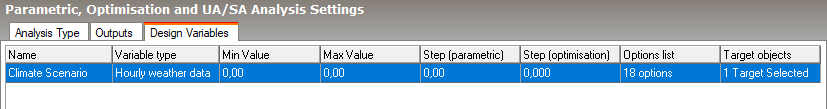
Step 5.d - On to the Design Variables tab.
Delete all but one variable from the list by selecting each in the grid in turn and pressing the Delete variable Info panel link.
You should now have only 1 item Design Variables list.
Select it and click on the Edit variable Info panel link.
On the Edit Analysis Variables dialog select the Hourly weather data Variable type (it can be found under the Location/weather/orientation category heading). Press OK.
Click on the Options list dialog option and then on the browse button to display a list of the available Hourly weather components. The 18 custom components should appear in red (since they were added as custom components). Select these 18 components by checking the checkbox to the left of each item and ensure that no other items are checked. Press OK.
When you press OK, a dialog appears to help you order the options list. In this example you may like to order them as follows:

Once you are happy with the order, press OK to accept and return to the Variables dialog.
Click on the Target objects dialog option and press the browse button to the right. Ensure that the Building is selected.
Select the Name field on the dialog and enter the name of the variable as "Climate Scenario". Press OK to close the Analysis variables dialog and return to the Variables tab of the Parametric, Optimisation and UA/SA Analysis Settings dialog, which should now look like this:
Press OK to confirm changes and close the Parametric, Optimisation and UA/SA Settings dialog.
Go to the Simulation screen and if the results are no longer available re-run an annual simulation. When the simulation is complete, click on the Parametric tab and click on the Update toolbar icon to open the Calculation options dialog.
Select the Output you would like to see displayed as simulation results are received back from the Simulation Manager (optional).
Once you have completed your review of the options press the Start button in the bottom right of the screen. The process will involve running 18 simulations which are run in parallel using the Simulation Manager. Once simulations are complete, close the Calculation options dialog.
Choose the Parametric output to display on the Display options panel to the bottom left of the main screen. You can choose to display either of the 80% or 90% acceptability criteria options.
Right click on the output graph and set the Plotting method to Bar. You may instead prefer the Horizontal Bar option to display the bars horizontally to ensure that the scenarios are written horizontally instead of sloped as they are when displaying vertical bars.
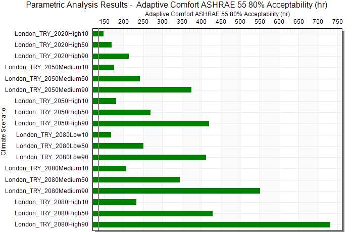
The results show the extent of discomfort in the model for each of the 18 future climate scenarios.