This tutorial will guide you through a more realistic uncertainty and sensitivity analysis for a post-occupancy application.
Problem: Identify the most influential factors impacting heating energy use in an office building by comparing uncertainty due to occupant behaviour and to construction quality.
Explanation: The example is based on the following assumptions:
The following are the variations that are to be applied for the two categories:
|
Category |
Input |
Variability |
|
Occupant behaviour |
Heating Setpoint |
Target setpoint = 20°C. Uncertainty is represented by normal distribution with a standard deviation of 1°C. Lower Bound = 18°C. Upper Bound = 21°C to maintain a 2°C dead band with cooling setpoint. |
|
Equipment Power density |
Target value = 13W/m2 Uncertainty is represented by triangular distribution Lower Bound = 10W/m2 to represent low IT usage work environment Upper Bound = 20W/m2 to represent a high IT usage work environment |
|
|
Construction Quality |
Infiltration |
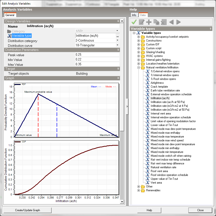
Target value = 0.25 ach Uncertainty is represented by triangular distribution Lower Bound = 0.22 ach* Upper Bound = 0.35 ach* |
|
Wall U-value |
Target value = 0.30 W/m2K Uncertainty is represented by Binomial distribution** Lower Bound = 0.25 W/m2K * Upper Bound = 0.45 W/m2K * |
|
|
Window U-Value |
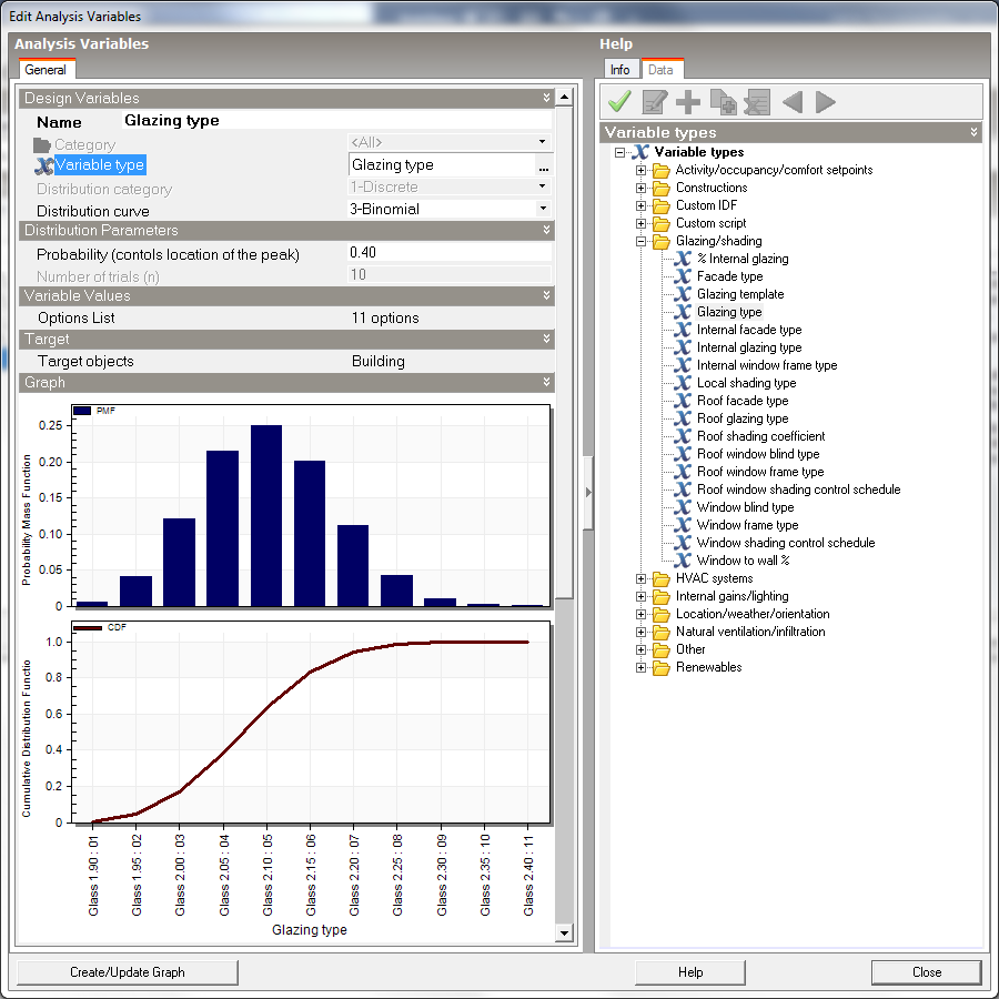
Target value = 2.00 W/m2K Uncertainty is represented by Binomial distribution** Lower Bound = 1.90 W/m2K * Upper Bound = 2.40 W/m2K * |
|
|
Roof U-value |
Target value = 0.20 W/m2K Uncertainty is represented by Binomial distribution** Lower Bound = 0.16 W/m2K * Upper Bound = 0.30 W/m2K * |
* Lower Bound values represent the instances when high degree of care was put on construction quality and targets were exceeded. This is less likely to happen and the over-achievement in normal practice would not be very high. On the other hand, Upper Bound values represent the instances when low care was put on construction quality and targets were not met. This is more likely to happen and in normal practice the deviation could be significant.
** Wall, roof and glazing U-values are not direct inputs in EnergyPlus, therefore the variation in U-value must be represented by creating a sequence of construction components to create fixed incremental increases in U-value. Then discrete distributions can be used to represent the variation.
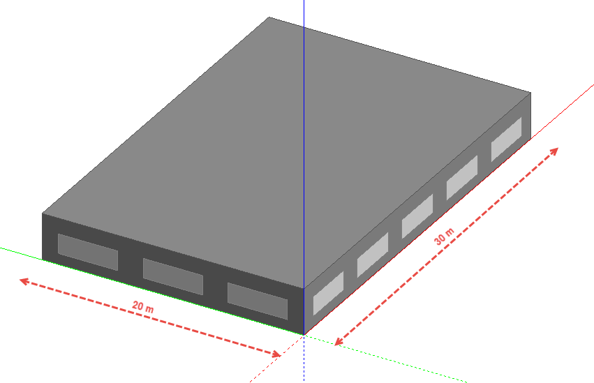
Create a new file located in London Gatwick and add a building to the site with a simple rectangular block having dimensions 30m x 20m as shown below. Use default Model options and template settings. DesignBuilder as supplied will use a Simple HVAC Fan Coil Unit system as the default. For this example, you should make sure that you have heating and cooling selected and no natural ventilation (this will be the case for a new model with an FCU HVAC system selected).
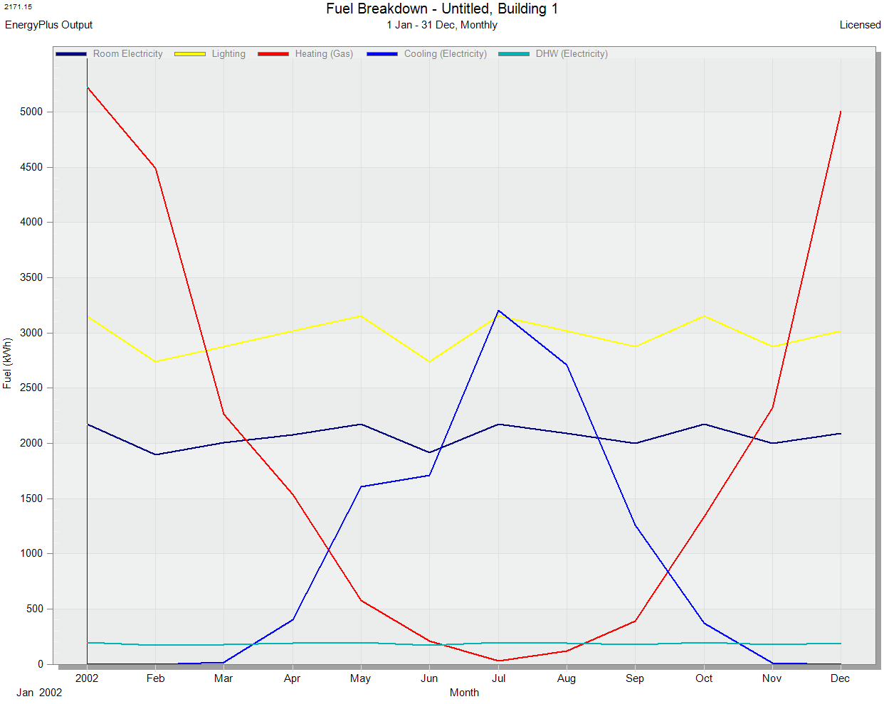
Click on the Simulation tab and run a base annual simulation. Because it is a simple model you can select hourly results. Make sure to also choose Monthly results which are required by the Optimisation. Check the hourly results for the simulation period and make sure that the model is behaving as expected, including temperatures within the building, operations periods etc. If not, adjust the model and repeat this step until you are happy with the base model hourly results. Monthly results should look something like the screenshot below.
Once you have a good understanding of how the base model operates, you are ready to start the uncertainty and sensitivity analysis stage. To do this click on the Optimisation + UA/SA tab of the Simulation screen. Because you don't have any results yet, the Parametric, Optimisation and UA/SA Analysis Settings dialog is displayed.
Change the Analysis type to 3-Uncertainty/Sensitivity as shown below.
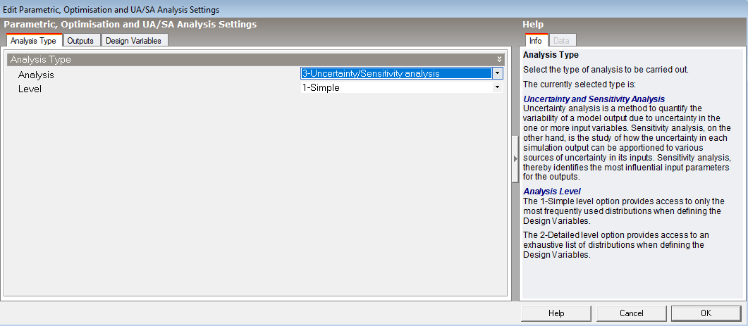
This will set up the rest of the tabs on the dialog and allow you to define the uncertainty and sensitivity analysis problem, i.e. what it is that you want to achieve from the uncertainty and sensitivity analysis study.
Use the following settings for this example to us identify:
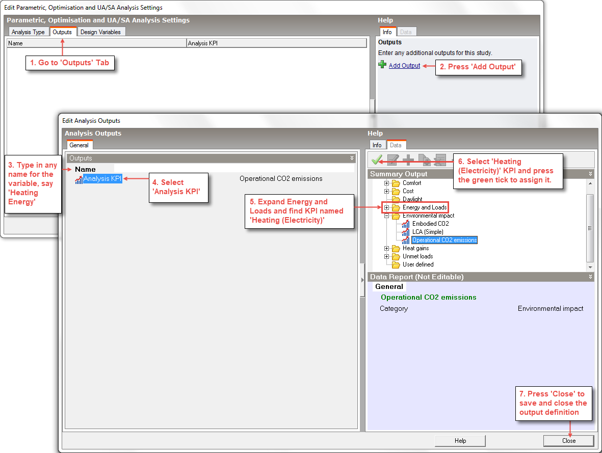
Add a new output by using the Add Output tool to access the Edit Analysis Outputs dialog. The procedure to select the Heating (Electricity) output is shown below.
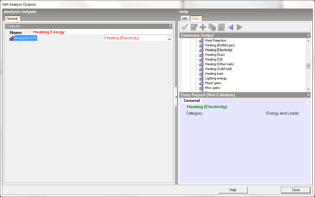
When finished, the Heating (Electricity) Analysis Output Dialog should look like this:
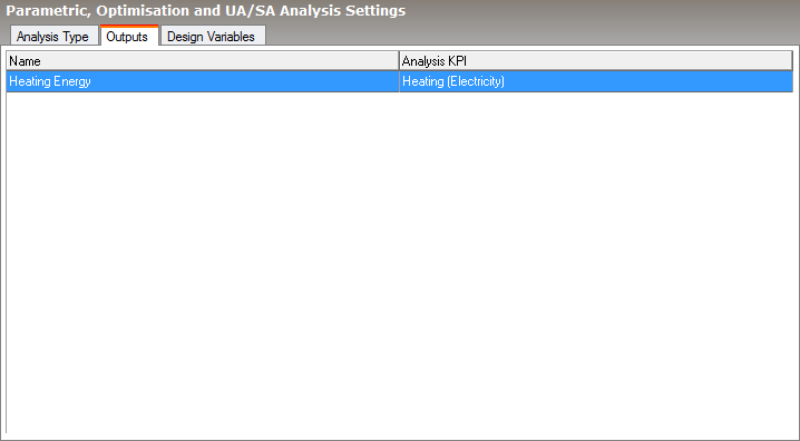
And when the Output dialog is closed the Outputs table should look like this:
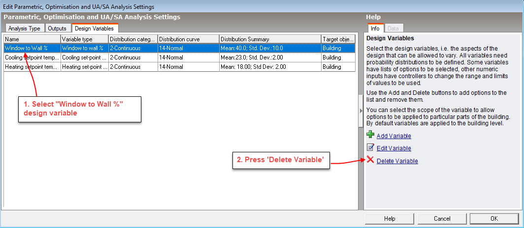
Go to the Design Variables tab. There are three pre-defined design variables. For this tutorial we need to remove the Window to Wall % design variable, modify the Heating and Cooling Setpoint variables and add 5 new variables.
1. To remove Window to Wall % and Cooling setpoint variables, follow the steps below:
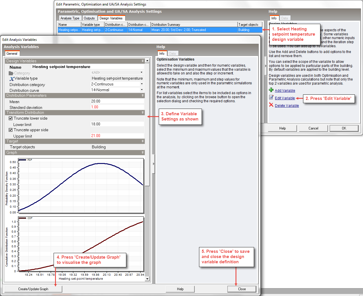
2. Edit the existing Heating setpoint temperature variable by following the steps described below:
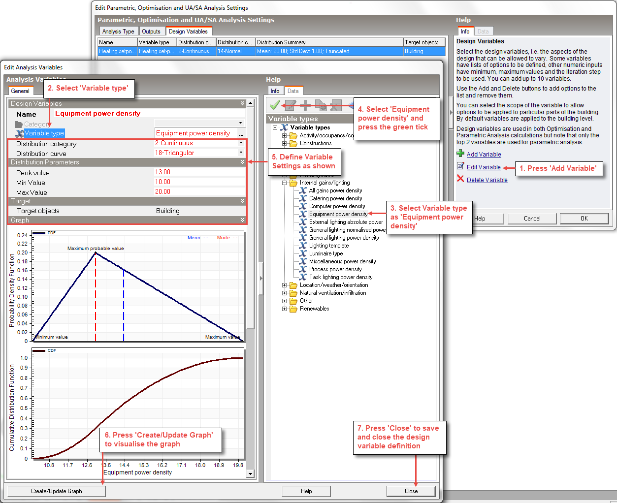
4. Add a new Equipment power density variable by following the steps described below:
5. Add a new Infiltration (ac/h) variable by following the steps described below:
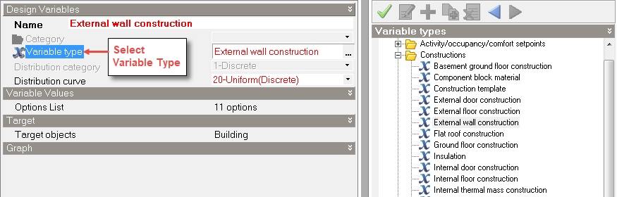
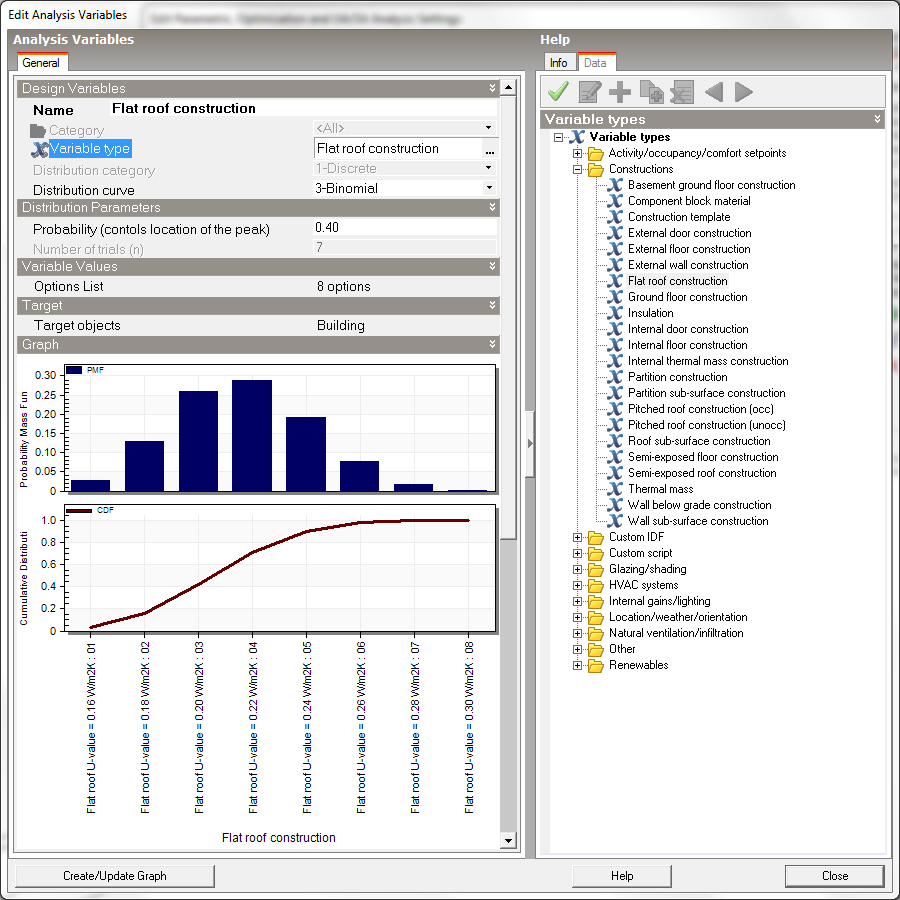
6. Add a new External Wall Construction variable by following the steps below:
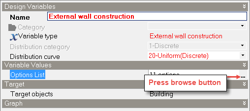
- Click on the Browse Button:
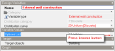
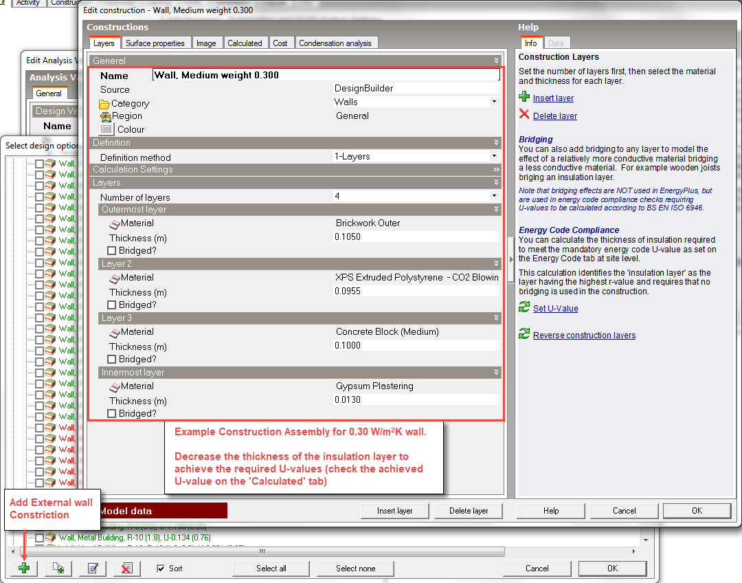
- Add a new construction for U-value of 0.30 W/m2K. Example shown below:

Note: You can use the Set U-value tool in the Info panel to achieve a specific U-value.
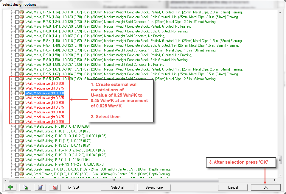
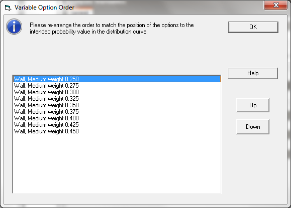
- Similarly, create 9 external wall constrictions of U-value of 0.25 W/m2K to 0.45 W/m2K with an increment of 0.025 W/m2K.
- Configure the options list to ensure that selection list is in order of increasing U-value order and press OK to close the dialog:
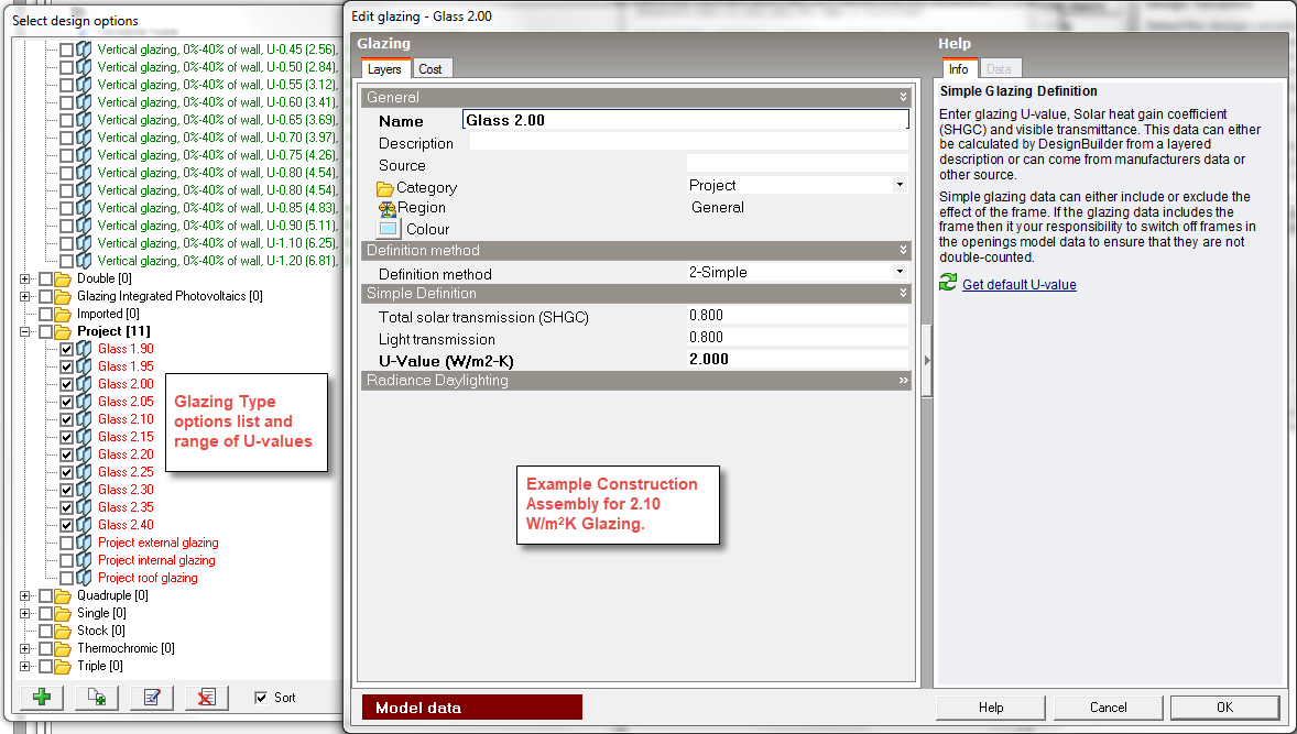
7. Similarly add a new Glazing type variable by following the steps below:
Note: Use the 2-Simple glazing Definition method where you can enter the U-value directly.
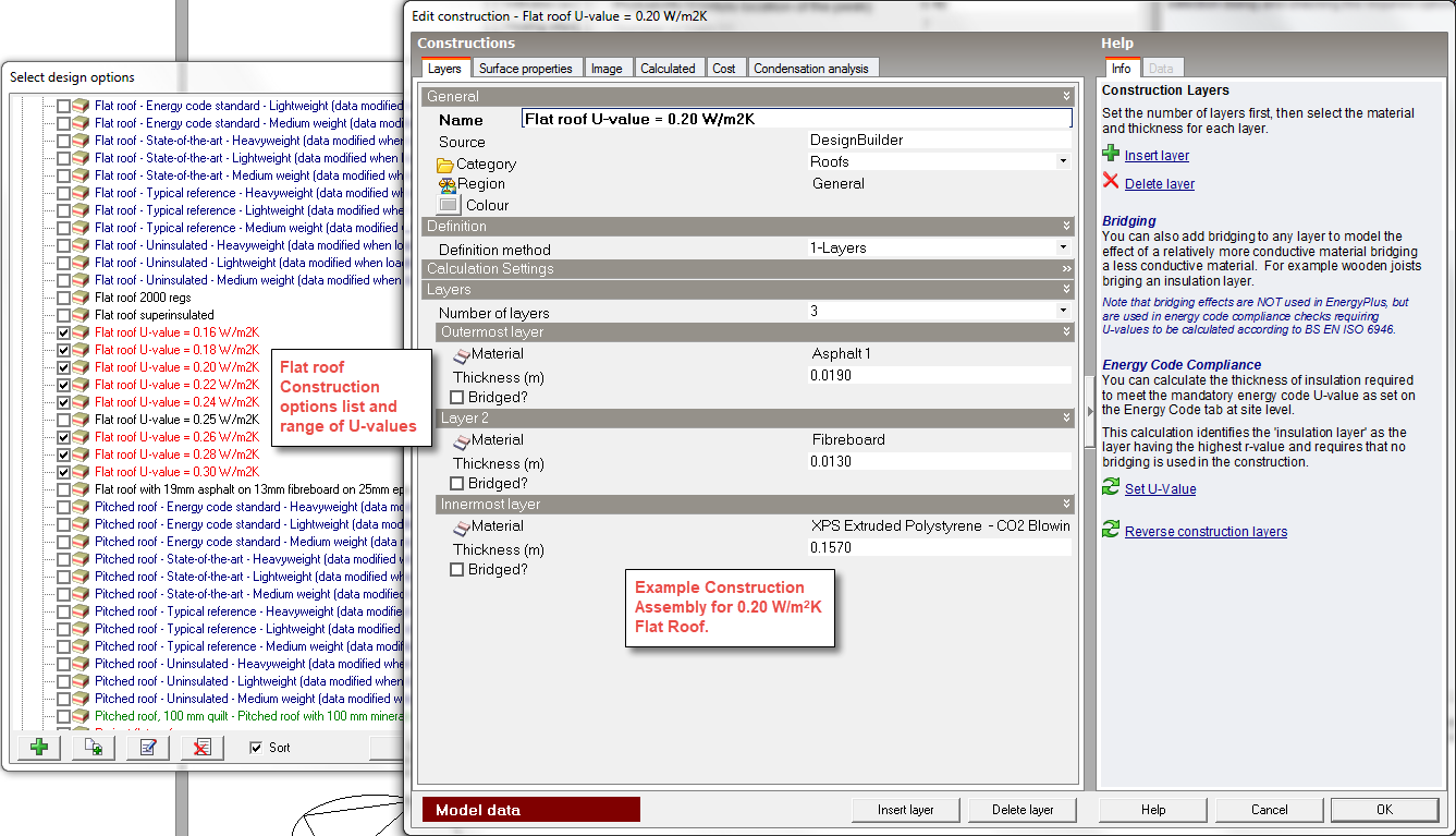
8. Similarly add a new Flat roof construction variable.
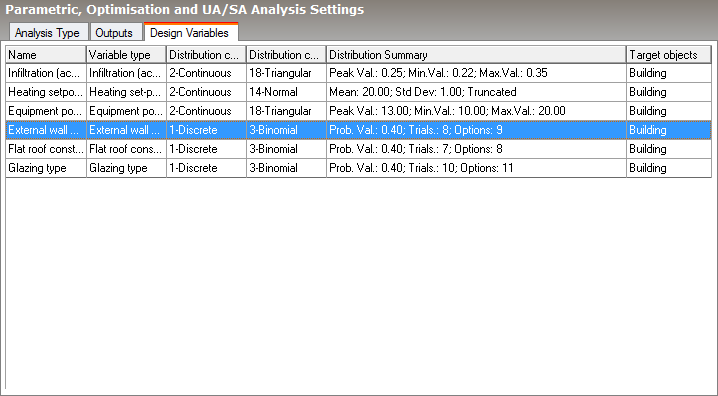
9. The final list of design variables should look like this:
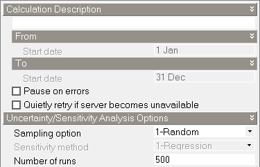
Having confirmed the uncertainty and sensitivity analysis options, the next dialog to open will be the Calculation options. Change the number of runs to 500 for this detailed analysis and, otherwise, use default settings.
Once you have completed your review of the options press the Start button in the bottom right of the dialog. The uncertainty and sensitivity analysis process will involve running a lot of simulations. With the recommended settings there will be 500 runs with 20 runs being plotted in each batch, updating the histogram as each batch is finished. That means that 25 batches will be run! For our simple office building this shouldn't take too long with the Simulation manager running the simulations in parallel. However, if time is an issue it is usually worth starting with a smaller number of runs.
During the runs uncertainty outputs are plotted at the end of each batch.
Note: While it is possible to stop the simulations before the UA/SA process is incomplete, this is not recommended as in this case uncertainty analysis results could be incorrect and sensitivity analysis results will not be created.
After all the runs have been finished an alert is displayed as shown in the screenshot below. Press OK to dismiss the alert and then Press Close to return to the Optimisation +UA/SA tab of the simulation screen to analyse the results.
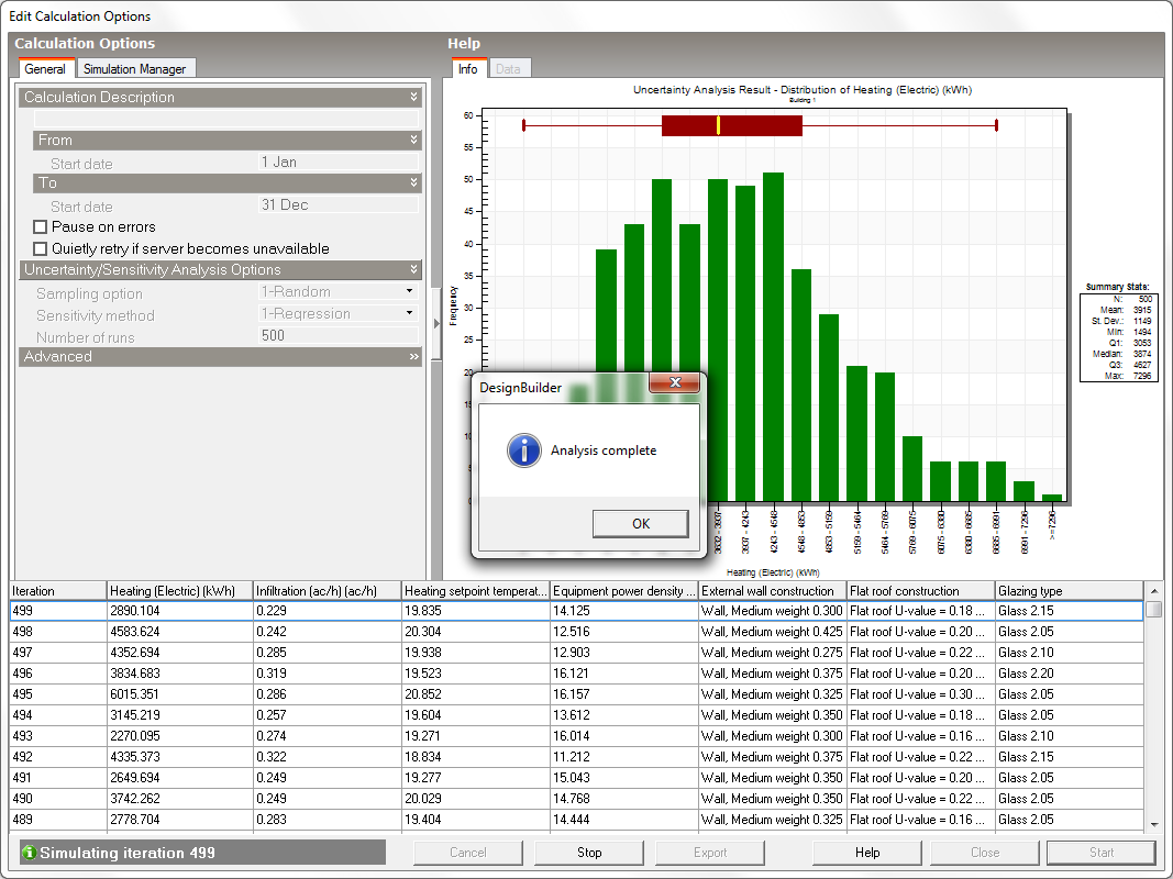
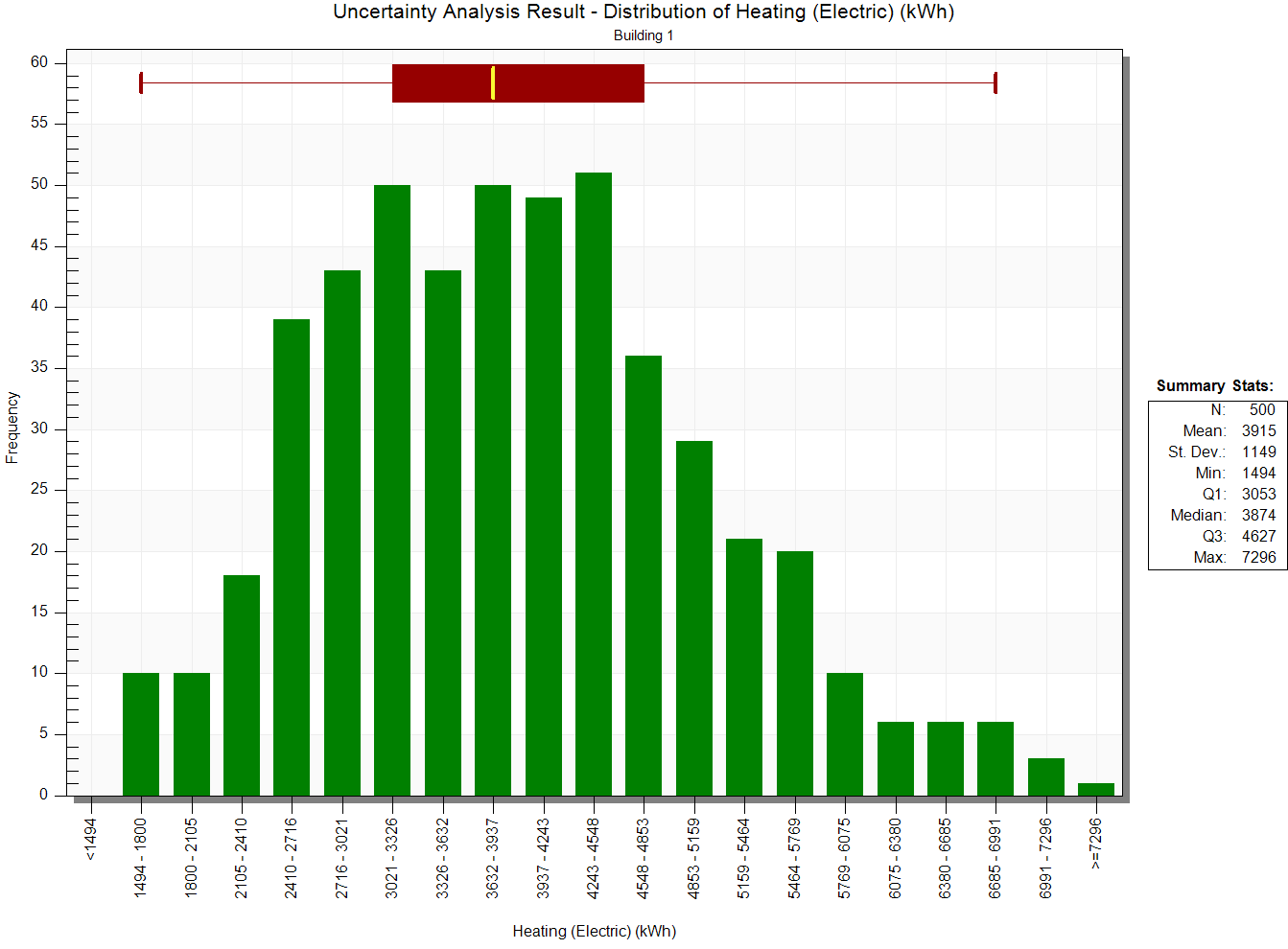
Keep the default 1-Uncertainty analysis Analysis type in the Display options panel result to view UA results first. You should be able to see from the histogram and summary statistics in the right hand panel on the graph that:
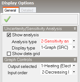
To visualise the sensitivity analysis results, change the Analysis type to 2-Sensitivity Analysis.
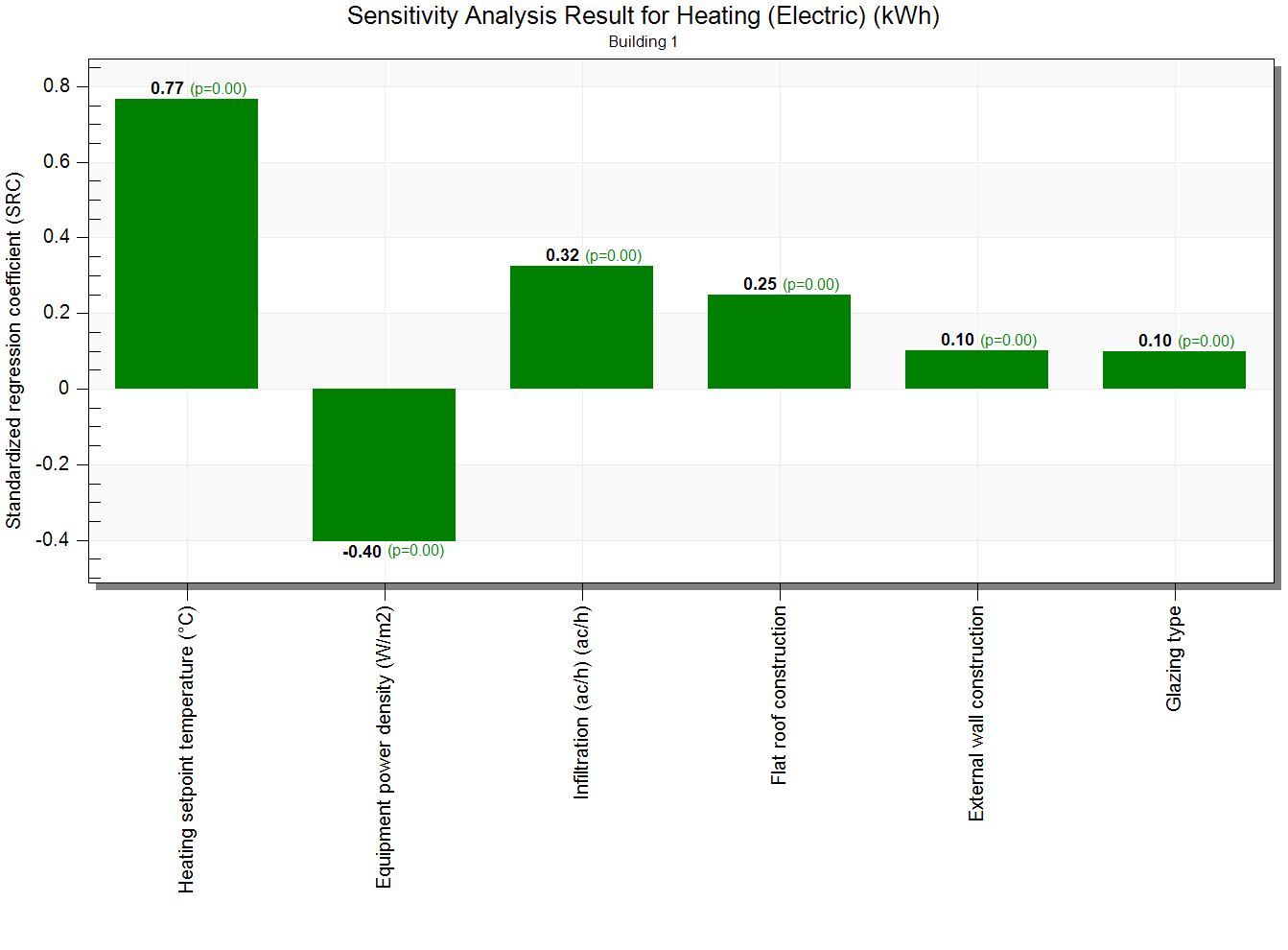
The Sensitivity analysis results are shown by default in decreasing order of importance with the most important variable on the left and the least important on the right. The value written above each bar in black bold is the standardised regression coefficient (SRC), telling us the relative importance of each input. In green to the right of each SRC value is the p-value. You should see in our example that the p-value for all inputs are 0. Note that a low p-value (<0.05) indicates a high level of confidence in the result for that variable.