This tutorial shows how to create a basic Custom Script KPI for an optimisation analysis with a Python script using the db_eplusout_reader library provided with DesignBuilder. It is based on an example problem to identify the set of design variations that lead to optimal building performance based on design objectives to minimise "Total system energy" consumption while at the same time minimising construction cost. DesignBuilder doesn't include a built-in "Total system energy" KPI so the tutorial demonstrates how to write a script to generate that output from the EnergyPlus results. The script calculates a project-specific definition of "Total system energy" by accessing 3 energy consumption output variables reported in the EnergyPlus SQLite output file, summing them and feeding the result back to DesignBuilder after each simulation to process as a KPI value.
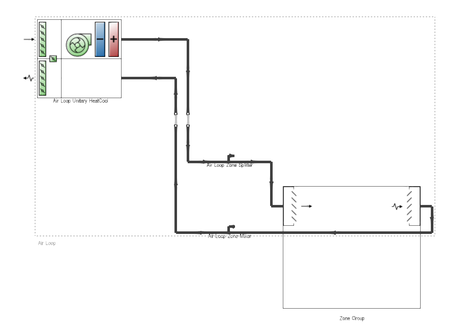
The model is the same base model used in the previous Optimisation Tutorial - Custom Script KPI Example 2 - Reading the EUI KPI Using EpNet (C#) and eppy (Python), but in this case it uses a Unitary Heat Cool HVAC system to allow EnergyPlus to calculate a realistic energy consumption value. Outputs for individual end uses are combined in the script to form the "Total system energy" KPI.
Optimal settings for Window To Wall %, Glazing type and Shading overhang length will be identified for the building that provide the lowest total system energy consumption while keeping construction costs as low as possible. Default building component costs and other settings are used throughout to allow us to focus on the Custom Script KPI.
The steps involved are as follows.
1. Create a new model located at London Gatwick.
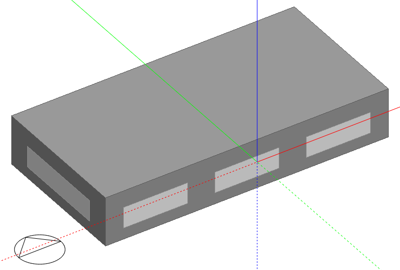
2. Add a building using default settings and draw a rectangular block measuring 20m by 10m with block height of 3.5m as shown below.
3. Load the Generic Office Area Activity template at building level on the Activity Tab.
4. On the Lighting tab at building level switch on Lighting control
4. On the Model options dialog set Detailed HVAC option.
5. Navigate to the <HVAC System> node and click on the Load HVAC Template toolbar icon. On the dialog select the Unitary Heat Cool template and press the Next button on the wizard.
6. Select the zone to be the control zone - in this single zone model it will be Block1:Zone1.
7. Press Finish to load the template.
8. The Unitary heat cool system is one of the simplest systems capable of maintaining comfortable conditions by heating and cooling multiple zones from a single AHU.
Click on the Simulation tab and run a base annual simulation. Because it is a simple model you can select hourly results. Make sure to also choose Monthly results which are required by the Optimisation process. Check the hourly results for the simulation period to ensure that the model is behaving as expected, including temperatures within the building, operations periods etc. Make any adjustments to the model and repeat this step until you are happy with the base model hourly results.
1. Open the Parametric, Optimisation and UA/SA Analysis Settings dialog by clicking on the  toolbar icon and set the Analysis type on the Analysis tab to 2-Optimisation.
2. Go to the Objectives tab and add 2 new objectives for construction capital cost and total system energy. You can either edit the existing objectives or first delete those and create 2 new objectives. The steps involved are described below.
To create the "Total system energy" objective, a new Summary Output (aka KPI) must be created. Click on the Objective KPI to open the list of existing Summary Outputs in the Info panel. Our "Total system energy" KPI won't be listed there at first, so create it now by clicking on the existing Custom Script Summary Output on the list of KPIs, click on the Create copy of highlighted item Info toolbar icon and edit the copy. Make the following settings on the Summary Output dialog.
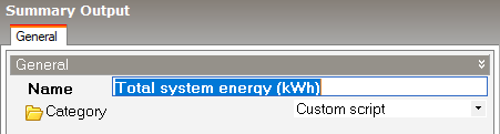
Note: The name entered here on the Summary Outputs dialog must match the name given in the custom script described below. You may like to copy the name and paste it somewhere safe where you can easily access it later when writing the script.
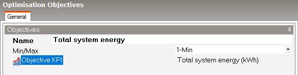
Save the newly created KPI and select it on the Optimisation Objectives dialog.
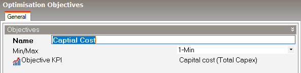
Name the objective "Total system energy". That name is for your own reference only and unlike the Summary Output name, it does not need to match anything else.
Select the 1-Min Min/Max option to say that you wish to minimise EUI. The dialog should now look something like the screenshot below.
Now create the cost objective. This is straightforward as we can use a standard KPI.
Select the Capital cost (Total Capex) KPI and call the objective "Capital Cost".
Select the 1-Min Min/Max option to say that you wish to minimise EUI. The objectives dialog should now look like the screenshot below.
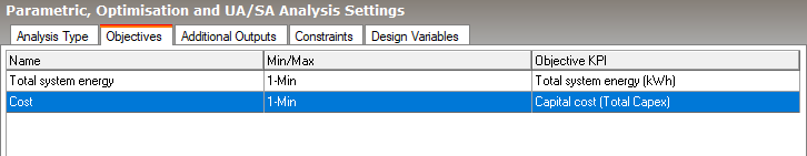
With both objectives defined, the Objectives tab should now be set up as follows:
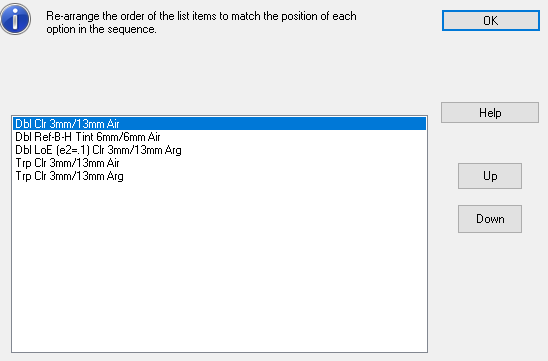
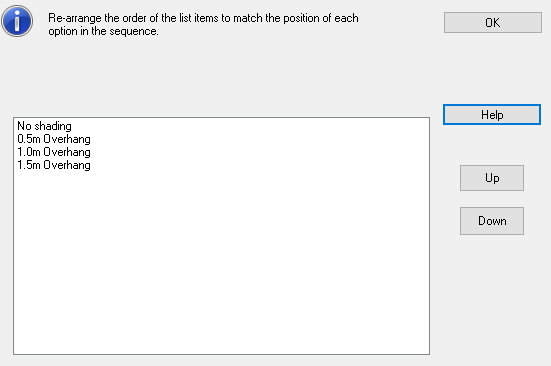
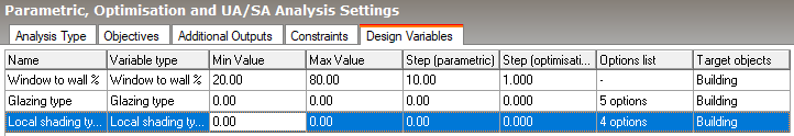
Now set up the design variables. The 3 variables to be included are:
With all 3 variables defined, the Variables tab should now be set up as follows:
The next task is to write the script that will read the simulation results from the ESO file, process them and pass back to DesignBuilder as a Custom KPI. Steps are as follows.
1. Click on the Scripts  toolbar icon to open the Script Manager dialog and click on the Enable scripts checkbox.
2. Click on the Script browse item. A list of the existing scripts appears in the Info panel to the right.
3. Click on the Python-Script category and press the Add new item Info toolbar icon to open the Edit script dialog.
4. Copy and paste the script below into the script window. In summary, the script works as follows. The key heating, cooling and system fan energy consumption outputs are loaded from the eplusout.sql simulation output file, summed to create a total and then written to the temporary "ParamResultsTmp" DesignBuilder results table used for the purpose.
from db_eplusout_reader import Variable, get_results
from db_eplusout_reader.constants import *
from datetime import datetime
# ensure that SQLite outputs are generated
def before_energy_idf_generation():
site = api_environment.Site
for building in site.Buildings:
building.SetAttribute("SSSQLiteOP", "1")
def after_energy_simulation():
file = api_environment.EnergyPlusFolder + r"eplusout.sql"
variables = [
Variable("", "Heating Coil Electricity Energy", "J"),
Variable("", "Cooling Coil Electricity Energy", "J"),
Variable("", "Fan Electricity Rate", "W"),
]
results = get_results(file, variables=variables, alike=True, frequency=RP)
convertJ_kWh = 3600000
convertW_kWh = 8.76
heating = results.arrays[0][0] / convertJ_kWh
cooling = results.arrays[1][0] / convertJ_kWh
fan = results.arrays[2][0] * convertW_kWh
system_energy_kWh = str(heating + cooling + fan)
site = api_environment.Site
table = site.GetTable("ParamResultsTmp")
record = table.AddRecord()
record[0] = "Total system energy (kWh)"
record[1] = str(system_energy_kWh)
Note: The heating and cooling coil electric energy variable outputs have been divided by 3,600,000 and fan power multiplied by 8.76 to convert the units from Joules to kWh and Watts to kWh respectively.
Tip: To save time you can copy the above script and paste it into the dialog. Note that Python requires the indentation as part of its syntax and when you paste the script the indents may become lost. In this case you must insert the indents manually after the paste. The easiest way to do that it by using the <Tab> key.
Tip: The DesignBuilderSoftware \ db-scripts Github repository includes the latest versions of the above script as well as other scripts used in DesignBuilder tutorials and examples.
Click on the Simulation tab and press update to re-run a base annual simulation.
Navigate to the Optimisation + UA/SA tab on the Simulation screen and press the Update toolbar icon to open the Optimisation Calculation Options dialog and make the following settings. These should be the same or similar to the defaults.
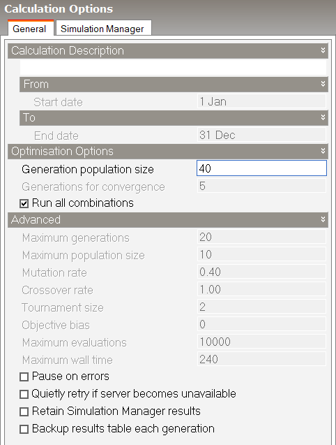
Press the Start button to run the optimisation simulations.
After the optimisation has converged and you have closed the Calculation Options dialog, you should see results similar to those below on the main screen.
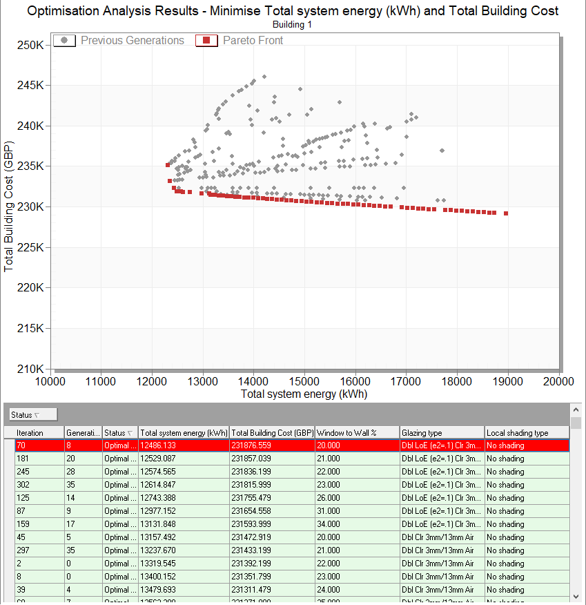
The optimisation results showing the trade off between Total energy consumption and capital cost will be dependent on the costs associated with the various building components, especially the glazing, external walls and overhang shading fins. Given the default costs used in this model, we can see that for a balanced energy performance at 12486 kWh, it necessary to spend 231,876 GBP for 20% WWR, double glazed low-e glazing with no overhangs.